Chris J. Topping
Dept. Wildlife Ecology,
National Environmental Research Institute, Aarhus University,
DK-8410, Roende, Denmark
15th October 2008, revised 27th September 2011
Overview
The ODdox documentation (Topping et al, 2010) is a hybrid between the ODD protocol (Grimm et al. 2006) for describing IBMs and Doxygen (http://www.doxygen.org) a standard software tool designed to increase the accessibility of program code. In ODdox documentation provides a set of html documents generated by Doxygen which form cross-linked documentation of all classes, methods and variables used in a progam code. This allows the user to browse through classes and see the inter-relationships in the code. At the lowest level the code is presented together with a brief description of what it does, and including the comments placed inside the code itself. The ODdox thus provides a powerful way of documentating IBMs and allowing others to choose to see precisely what has been done or to get an overview quickly without the details.
This version (1.1) of the vole documentation corresponds to the model version used to evaluate the impact of landscape and predator characteristics on vole cycling and is post 2011 pattern oriented modelling testing. Predator details can be found in the TPredator class, for landscape information please see the overall ALMaSS documentation available at http://www.almass.dk
1. Purpose
The field vole model was developed as part of the ALMaSS framework (Animal Landscape and Man Simulation System) which was primarily constructed as an assessment tool for use in answering management and policy questions related primarily to changes in farm management, landscape structure and land use. The ALMaSS system was designed to be as flexible as possible since the precise applications of the system were not known in advance. The field vole model is therefore designed to be a flexible model capable of translating changes in it's simulated environment into patterns of changes in population sizes, reproductive outputs and distribution with time. Flexibility is a function of the high level of detail implemented in the model with the aim of simulating Microtus agrestis responses as realistically as possible, whilst still maintaining a manageable code volume and parameter space.
2. State Variables & Scales
2.a Vole Base
- Attribute: Vole_Base::m_Age The age of the object in days.
- Attribute: TAnimal::m_Location_x The x coordinate in the landscape where the individual were born.
- Attribute: TAnimal::m_Location_y The y coordinate in the landscape where the individual were born.
- Attribute: Vole_Base::IDNo Identification number associated with the object.
- Attribute: Vole_Base::m_Sex Male or female.
- Attribute: Vole_Base::m_Mature Boolean variable indicating whether the vole has reached maturity (==true).
- Attribute: Vole_Base::m_TerrRange The radius of their territory.
- Attribute: Vole_Base::m_LifeSpan Maximum number of days left for the vole to live if not subject to other mortality.
- Attribute: Vole_Base::m_Weight Weight of the vole in grams.
- Attribute: Vole_Base::m_DispVector The current dispersal direction.
- Attribute: Vole_Base::m_Have_Territory Boolean variable set to true if they have a territory.
- Attribute: Vole_Base::CurrentVState Behavioural state of the object.
- Attribute: Vole_Base::m_pesticideInfluenced For specific pesticide use only.
- Attribute: Vole_Base::m_pesticideInfluenced2 For specific pesticide use only.
2.b Vole Female
- Attribute: Vole_Female::m_NoOfYoung Number of young in the nest.
- Attribute: Vole_Female::m_Pregnant Boolean variable set at true if the female is pregnant.
- Attribute: Vole_Female::m_DaysUntilBirth Number of days until the female gives brith.
- Attribute: Vole_Female::m_YoungAge The age of the young produced.
- Attribute: Vole_Female::m_BornLastYear Receives the value of 1 if she was born the previous year.
2.c Vole Male
- Attribute: Vole_Male::m_fertile Indicates the fertility status of the male. Default is fertile == true. Used primarily in pesticide applications. Administrative state variables used to speed of facilitate operation of code:
- Attribute: Vole_Base::m_OurPopulation Pointer to the population manager. This is needed by all individuals to access population manager functions.
- Attribute: Vole_Base::SimW Provides the individuals with the width of the landscape.
- Attribute: Vole_Base::SimH Provides the individuals with the height of the landscape.
2.d Habitats
ALMaSS is spatially explicit and has a square raster GIS based representation of a landscape with a default resolution of 1 m2. The size of the landscape can change with the scenario simulations and can be in the scale of e.g. 10 km x 10 km; 5 km x 5 km or 1 km x 1 km to make the model flexible and applicable to a wide variety of scenarios and data availability. The length of a simulation run is flexible as well and can be set to any number of years with the time-step set at one day as a default. This resolution and extent make it feasible to model vole behaviour at a fine scale whilst still keeping run-times within sensible bounds.
State variables used by the vole model and associated with each habitat unit were:
- m_polyrefs Identification number associated with each unique polygon.
- m_elems Land-cover code for each polygon.
- m_farms If the code for the land-cover were a field then a farm owner was associated with it and carried out farm management on the owned units.
- m_vege_type Vegetation type for the polygon (if any vegetation grows in the polygon.
The landscape model in ALMaSS was weather dependent and the state variables associated with the weather sub-model were:
- m_temptoday Mean temperature on the given day (Celsius).
- m_windtoday Mean wind speed on the given day (m/sec).
- m_raintoday Total precipitation on the given day (cm).
The ALMaSS Landscape component is responsible for handling all landscape, weather and management related sub-models. These include 74 management plans for Danish crops, crop and habitat related vegetation and insect growth models, and miscellaneous human management models. Documentation of these is outside the current scope of this documentation, but please refer to the following documentation: 13-17.
3. Process Overview and Scheduling
The field vole model consists of three life-stages; juvenile, female and male separated into two classes of males and females. During a life-cycle the vole object transitions through a number of behavioural stages based on information obtained during its current behavioural stage and messages received from other objects in the simulation. This scheduling together with many other functions are contained in the Vole_Population_Manager class (see submodels). The voles enter the simulation at the location of the females nest and at 14 days of age (WeanedAge==13) (Innes and Millar, 1994; Leslie and Ranson, 1940) as either a female or male with m_Mature == false. They will enter the state of Vole_Female::st_Evaluate_n_Explore (female) or Vole_Male::st_Eval_n_Explore (male) and start searching the area for a suitable territory.
Every new day for a vole in the simulation starts off by evaluating and exploring (Vole_Female::Step Vole_Male::Step dependent on their sex). Other behaviours may ensue dependent upon the information gathered during this process. Possession of a territory is a prerequisite to breeding. Males have the possibility of breeding with any females with territories located totally or partially within the male?s territory. Voles that find themselves in older voles territories of the same sex with an overlap of >50% must move. The criteria for assessing territory quality vary with season, and for the male in the breeding season include the proximity of females.
3.a Scheduling
The simulation time-step is one day, meaning that at the end of each day the state of the simulation is consistent with all objects having completed one day of activity. All farming and other human activities are assumed to occur at the beginning of the day on which they are scheduled, thus knowledge of these events is available for all animal models which are considered subsequently.
A hierarchical approach to scheduling of animal objects is used to overcome the problems of currency between interacting objects discussed by Topping et al. (1999). Although the computer is operating serially, the objects must be scheduled such that they appear to operate in parallel. For the vole model and all other ALMaSS models this is achieved using a state machine to move objects between behavioural states and by dividing the time-step into three sections, namely BeginStep, Step and EndStep. BeginStep all objects execute their BeginStep code before any objects can execute Step code. All male objects are called in a random sequence and execute the step code, then all females also in a random sequence. When all male and female voles are finished with BeginStep this process is then carried out for Step. There is a significant difference between Step and BeginStep and EndStep. In Step a vole must signal that it is finished with Step behaviours for this day otherwise after the first pass through all individuals, a second pass is carried out for those individuals that have not indicated that the Step is done with. This process is repeated until all individual objects are finished with the Step code. At this point the EndStep is called in the same way as BeginStep.
The BeginStep/Step/EndStep structure allows for a very flexible combination of interlinked behaviours (although only used to a limited extent by the vole), and permits efficient use of resources e.g. by removing dead voles in the BeginStep or EndStep before they waste CPU resources in Step. Handling of all scheduling via BeginStep/Step/EndStep is performed in the base class Population_Manager.
3.b Vole States
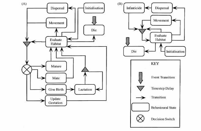
The figure above shows the overall structure and relationships for the female (A) & male (B) behavioural states. Details of the these states are provided below together with direct links to the program code to facilitate understanding of the way in which states and transitions are used.
3.b.i Evaluate & Explore
For the females, if the vole does not possess a territory (m_Have_Territory == false) or if the habitat quality in the current territory falls below Vole_Base::m_MinFVoleHabQual the vole will undergo dispersal (Vole_Female::Dispersal). If habitat quality is not below this threshold the vole will carry out an exploratory movement in one randomly picked direction (see Movement), to assess the habitat quality of a nearby area. If the habitat quality in the new area is greater than the old territory then she will move.
The male vole behaves the same way using Vole_Base::m_MinMVoleHabQual as the threshold level for dispersal outside the breeding season. Inside the breeding season, however, the vole also evaluates the proximity of females as a resource as well as the potential that he is in a larger (older) male's territory. If in an older male's territory then he will disperse, but he may also do this if there are no females present. The probability of this is given by the input parameter cfg_VoleFemaleMove (held in g_NoFemalesMove).
This simulates a seasonally territorial system, where the territoriality breaks down outside the breeding season as described by Erlinge et al. (1990) and Agrell et al. (1996).
Uses: Vole_Base::AssessHabitat, Vole_Base::CalculateCarryingCapacity, Vole_Base::CalculateCarryingCapacity.
3.b.ii Infanticide
- Vole_Male::st_Infanticide If the male has moved beyond the bounds of his original territory and established in a new area he will attempt to kill all new born voles within his new territory. In this way he will increase his reproductive access to females in the new territory (Agrell, 1998). The probability of killing the young is dependent upon their age and to what extend the female defends her nest. Infanticide figures for the field vole have not been available hence values from the study of Heise and Lippke (1977) on the closely related common vole (Microtus arvalis) have been used (Table 1).
3.b.iii Maturation
- Vole_Male::st_Maturation
- Vole_Female::st_BecomeReproductive A young vole will become mature when it attains the age of maturation during the breeding season (Table 1). When it is mature it is capable of mating once it has established a territory. Vole_Male::st_JuvenileExplore Ensures that the young male voles start to move away from the nest on the first day of independent life.
3.b.iv Dying
- Vole_Base::st_Dying The vole can reach this stat by three routes 1) it may be killed by a predator; 2) by external factors e.g. farm operations or traffic; 3) or it may reach the end of its life span (Table 1). Farm management as an external mortality factor cause death to the voles by the disturbance of grazing life-stock (25%), harvest and cutting (50%) and soil cultivation (75%). In all cases only those voles present on the field under farm operation at the time the management was carried out were subjected to agricultural mortalities. For other mortalities these are primarily connected to death as a result of dispersal or predation. Predatation can be by speficied predators e.g. Weasel or Owl, or in the absence of these in hte model as a function of background mortality controlled by the input parameter cfg_VoleBackgroundMort (g_DailyMortChance). NB POM fitting determined that the background mortality of adult males with territories needed to be lowered by 50% compared to females, hence adult male mortality is held in g_DailyMortChanceMaleTerr.
3.b.v Mating
- Vole_Female::st_Mating A female will mate if she mature during the breeding season and has established a territory. If the territory of a male is overlapping the females position she will be mated. If more than one males territory is overlapping her position she will be mated with the male closest to her location and gestation will start, which for the field vole last for 21 days (Leslie and Ranson, 1940; Innes and Millar, 1994). During mating a copy of the males genome is passed to the female and stored until used when any eventual offspring are weaned. Gestation Vole_Female::st_UpdateGestation Counts down the days of gestation and implements any reproductive impacts associated with pesticide accumulation (if any).
3.b.vi Give Birth
- Vole_Female::st_GiveBirth The number of young is adjusted to the age of the mother and the month of the year they are delivered as observed by Andera (1981). Gestating females which have been over-wintering will produce a higher number of young than females reaching maturity within the same year as their birth (Table 1). The gender of the young is determined by random allocation based on the assumption of an even sex ratio (Myllyimaki, 1977). Young will only be produced by females with good body condition (assumed equivalent to three days spent in a territory with HQT above (M/)FHabQualThreshold2 (i.e. above marginal).
3.b.vii Lactation
- Vole_Female::st_Lactating The female will enter this state when she has given birth. She will locate the best habitat within her territory to place her nest. She will stay within a radius of 6 m of the nest and feed her young (Jensen and Hansen, 2001). After lactation is over (i.e. the young are weaned) the female will do the special evaluation and explore as described in the section Special Exploration. The young produced at this point will carry a genome dependent upon a recombination of the male and female genes (the males genome was stored on mating). Recombination is controlled by void GeneticMaterial::Recombine and mutation can occur at this point depending upon the genetic settings used (outside the scope of this description).
3.b.viii Special Exploration
- Vole_Female::st_Special_Explore This behaviour is called after weaning of a litter when the female needs to expand her territory again. This does not use the Dispersal function so avoids extra mortality at this point and simulates the real phenomenon of sudden increase in daily home range after weaning (Agrell, 1995). In this case the exploratory movement is carried out in all eight directions rather than the daily single directional explore done in Exploration above.
3.c Important Methods
3.c.i BeginStep
- Vole_Male::BeginStep
- Vole_Female::BeginStep The BeginStep one of the three time-step divisions. This is called once for each vole before Step and EndStep. The main function here is to remove voles that die before they take up CPU resources in the Step code. It is also be used to check for pesticide accumulation levels in pesticide simulations.
3.c.ii Step
- Vole_Male::Step
- Vole_Female::Step The Step is one of the three time-step divisions. This is called repeatedly after before Step and before EndStep, until all voles report that they are done with Step. Most of the behaviours are controlled by moving voles between behavioural states in Step (for other models this is also done in BeginStep and EndStep). When a vole is done for the day it will signal this by setting StepDone==true. NB that a call to one behaviour may trigger a call to another behaviour on the next call to step inside the same time-step. In this way a daily cycle of activity can be undertaken (e.g. do reproduction and explore in the female).
3.c.iii EndStep
- Vole_Male::EndStep
- Vole_Female::EndStep The EndStep one of the three time-step divisions. This is called once for each vole after BeginStep and Step. The main function here is to remove voles that have died during step and otherwise to grow if not at max weight. Vole EndStep also checks if the vole was killed due to human management and determines the potential territory size. For newly adult voles the territory size will be set to the minimum size and grow larger until the vole has reached the maximum weight (Table 1). Male territory is generally larger than the females and a larger vole is capable of sustaining a larger territory (Agrell et al., 1996; Erlinge et al. 1990).
3.c.iv Movement
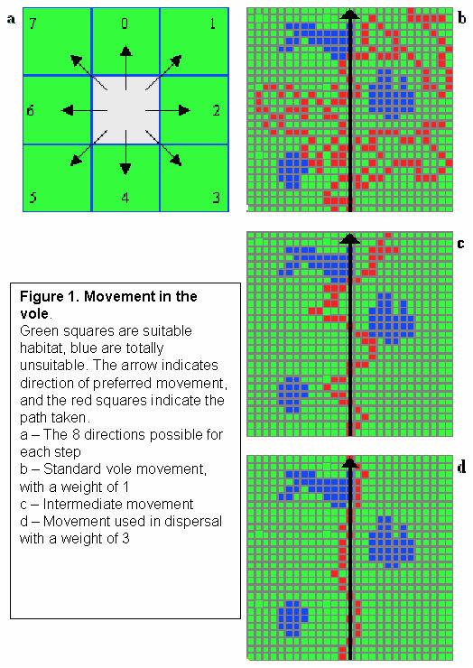
- Vole_Base::MoveTo Movement is an essential and difficult concept to model in an ABM. In ALMaSS, a standard method of implementing terrestrial movements was used and was defined by three parameters: 1) A directional vector, indicating the preferred direction. 2) A weight, indicating the strength of the bias towards the directional vector. 3) The number of steps, indicating the maximum allowed distance per time step.
Weights varied between zero (all eight directions allowed) and four (only the preferred direction allowed). For each step, habitat quality was evaluated in each of the possible directions and movement occurs to one of the suitable locations chosen at random. Different combinations of the movement variables resulted in a diverse set of potential animal-movement patterns across a landscape. Animals followed the above rules unless they became stuck, whereby the preferred direction and vectors would lead them into unsuitable habitats. In this case, the vector is altered by plus/minus one until movement is again possible. This basic movement model was enhanced by the addition of preferential choice between suitable habitats. Thus, the vole only makes a random decision if there is more than one location where the habitat quality is highest. This enhancement also requires a fourth parameter that describes the chance of an animal accepting a suitable, but not the most suitable habitat, to move to. This allows the animal to restrict its movement across some unsuitable habitats e.g., roads, but occasionally to cross them.
The problem of voles getting stuck is avoided by preventing backwards movement, but allowing the vector to change by +/-1 if there is no legal choice of habitats to step onto given the current vector and weight.
Uses: Vole_Base::MoveQuality, Vole_Base::MoveTo, Vole_Base::DoWalking & Vole_Base::DoWalkingCorrect
3.c.v Dispersal
- Vole_Base::Escape
As movement but with the weight of the directional vector set at three. In this way the vole is able to travel further away from the starting point than by entering the movement state.
| Parameter Name | Value | Source |
| Male Reproductive Start VolePopulationManager.cpp::cfg_GrassStartGrowth | 2 weeks after the grass starts to grow | Myllyimaki (1977); Jensen and Hansen (2001). |
| Day at which reproduction will no longer be restarted cfg_vole_reprofinishdate | Day 242 for Finland (POM fitted) | Estimated from Erlinge et al. (1983) |
| Max male territory (radius m) cfg_MaxMaleTerrSize | 20 | Agrell et al. (1996) |
| Max female territory (radius m) cfg_MaxFemaleTerrSize | 16 | Erlinge et al. (1990) |
| Min male territory (radius m)\ cfg_MinMaleTerritorySize | 12 | Erlinge et al. (1990) |
| Min female territory (radius m) cfg_MinFemaleTerritorySize | 8 | Jensen and Hansen (2001) |
| Infanticide risk by age Vole_all.cpp::InfanticideChanceByAge | % mortality with 1-9 days old {97,86,75,64,54,43,32,21,11} | Heise and Lippke (1997) Microtus arvalis |
| No of young (depending on year of birth and the month) Vole_Population_Manager::ReproTable | Female born this year {0,0,0,0,4,4,4,4,3,2,3,0}/n Female born last year {0,0,4,4,5,5,5,5,4,4,0,0} | Andera (1981) |
| Max female movement (m) Vole_all.cpp::FemaleMovement | 50 | Jensen and Hansen (2001) |
| Max male movement (m) Vole_all.cpp::MaleMovement | Max movement m with age in months{10,40,70,110} | Jensen and Hansen (2001) |
| Gestation period (days) Vole_all.cpp::TheGestationPeriod | 21 | Leslie and Ranson (1940), Innes and Millar (1994) |
| Weaned age (days) Vole_all.cpp::WeanedAge | >13 days old | Leslie and Ranson (1940), Innes and Millar (1994) |
| Weight at weaning (g) Vole_all.cpp::WeanedWeight | 5 | Myllyimaki (1977) |
| Max male weight (g) Vole_all.cpp::MaxWeightM | 60 | Myllyimaki (1977) |
| Max female weight (g) Vole_all.cpp::MaxWeightF | 55 | Myllyimaki (1977) |
| Growth per day (g) see Vole_Male::EndStep | Assumed linier growth, taking 90 days to reach maximum weight from weaning. | 90 days is estimated from Myllyimaki (1977) to be the time required during the growth period to attain max size. No growth was assumed to occur during over-wintering. The curve was linearized for speed of calculation. |
| Minimum male reproductive age (days) cfg_MinReproAgeM | 29 | POM fitted |
| Minimum female reproductive age (days) cfg_MinReproAgeF | 23 | POM fitted |
| Maximum life-span (days) Vole_Base::m_LifeSpan | 14 to 20 months | Myllyimaki (1977) |
| Extra daily mortality probability during dispersal cfg_extradispmort | 0.055 | POM Fitted |
Tabel 1. Overview of the parameters in the vole model with presented together with source information.
| Type | Vegetation Characteristics | Typical Landscape Elements | Habitat Score |
| Optimal habitat | Cover > 80%, height > 40 cm | Ungrazed and uncut grassland, old set-aside, field and road margins | 3 |
| Sub-optimal habitat | Cover > 40%, height > 10 cm | Young tree plantations, cereal crops undersown with grass, dry meadow or heathland | 2 |
| Marginal habitat | Cover < 40% or height < 10 cm | Grazed or cut grassland, cereal and grass crops | 1 |
| No habitat | No grass | Roads, mature tree stands, other areas with no grass | 0 |
| Non habitat | None | Buildings, water bodies | -1 |
Tabel 2. Vole habitat quality categories based on the study of Hansson (1971 & 1977).
Design
4. Design Concept
4.a Emergence
Emergent properties described by individual based state variables are: Weight. Territory size. Location (coordinates). Other emergent individual properties are: Distance moved by individuals. Realised lifespan. Individual genome. Individual location (habitat type) Reproductive output and success. Higher order emergent properties: Spatial distribution of voles. Population size and fluctuations. Sex ratios. Population reproductive output and success. Population genome.
4.b Adaptation
Vole movement in evaluate and explore and dispersal will provide the voles with a way to improve their basic fitness by optimising their territory quality, and maximising search range if territory quality falls. The infanticide behaviour of the male vole will improve genetic fitness.
4.c Fitness
Fitness is measured directly in terms of physiological reserves, size and the number of starvation days. Indirectly in the number of offspring a vole contributes to the population.
4.d Prediction
Prediction is not used by the vole.
4.e Sensing
Voles can sense the location of other voles, the age and territorial state of other voles, and their sex. They can also sense the type and structural quality of vegetation at their location. Interaction Voles interact in determining their territory locations, and breeding partners. There are also interactions between males attempting infanticide and females with young. Voles interact with predators and external events such as ploughing, harvest or mowing leading to their death. Onset of breeding is dependent upon vegetation growth, which is in turn dependent upon weather.
4.f Stochasticity
Stochasticity is built into the simulation at many levels. At the higher level there is the order in which voles are selected to carry out BeginStep/Step/EndStep actions. At a lower organisation level mortalities are probabilities and are implemented as a proportion e.g. the chance of ploughing mortality is 0.75 and is independently applied for each individual affected. Note however that although the chance of being killed e.g. by harvest is a probability (1 in 4), the vole will only be in a position to be subjected to this probability if it is in a field at the time the harvest operation is carried out. This is therefore deterministic in terms of the voles exposed to the causal event, but a stochastic mortality at the individual level for those so exposed.
Movement also relies of probabilities of stepping from one type of habitat to another e.g. a probability of making a mistake and taking a suboptimal step, but also where two steps are equally good, then the choice is stochastic. Infanticide is based on a probability scaling with the age of the young.
4.g Collectives
The only collective that exists is that used to describe the young in the nest before weaning, although this does not have class status, it is a data construct of by the female.
4.h Observation
The PopulationManager class is the primary route for observation of the simulation. All population managers have specialised states before and after all BeginStep/Step/EndStep parts of the time-step that can be used for output. Standard ALMaSS outputs include total population size, spatially related population size via habitat type, location, farm types or vegetation types; genetic information at the individual and population level, spatial information at the population level. In addition specialised observational probes can be written to extract specific information at global or local scales (e.g. number of voles affected by pesticide toxicity). All data can be temporally referenced, and additional visual output is available in the GUI version of ALMaSS.
For examples of vole outputs see Vole_Population_Manager::ImpactedProbe, Vole_Population_Manager::TheCIPEGridOutputProbe, Vole_Population_Manager::TheRipleysOutputProbe, Vole_Population_Manager::TheReallyBigOutputProbe.
5. Initialisation
As far as the voles are concerned initialisation occurs by random allocation of a pre-determined number of adult male and female voles into the landscape. Voles enter the landscape with a random age between 1 & 500 days, a weight of 40g and as mature individuals with no territories. For some genetic simulations and some ecological or behavioural questions it is also possible to delimit the areas voles are started in. The landscape is initialised by running a burn-in year without the voles to allow all management plans to start off at a realistic time.
6. Inputs
Input parameters vary with each application of the ALMaSS vole model but cover these basic types: 1) Landscape structure. Implemented as a GIS map, converted to ALMaSS data structures. Input fields consist of landscape element type (e.g. field, road, hedge) and extent. 2) Climate data on a daily basis. This data is looped if the simulation is longer than the data set. Data consists of mean daily temperature, daily precipitation and mean daily wind-speed. 3) Values for vole model parameters see tables 1 & 2. 4) Farming information this depends on the type and location of the farms being modelled and is implemented as a crop rotation and a set of management plans covering each crop used. These plans determine the timing and order of farm events, but these are in turn dependent on weather and farmers choices (both stochastic and mechanistic). 5) Other values related to specific application e.g. pesticide usage, toxicity, or timing of population crashes (e.g. see Vole_Population_Manager::Catastrophe).
7. Interconnections
The vole model relies on the ALMaSS system for a host of services and data relating to the simulated vole environment. A key component of the vole model is the Vole_Population_Manager. This class is responsible for managing lists of voles in the simulation and has a number of interface functions relating to passing information to and from voles:
- Vole_Population_Manager::SupplyOlderFemales - Returns false if there is an older female within the area p_x,p_y +/- range.
- Vole_Population_Manager::SupplyHowManyVoles - Counts vole positions on the map from within a specified range of an x,y, coordinate.
- Vole_Population_Manager::SupplyGrowthStartDate - Returns a day in the year that the grass started to grow, if it is growing. See also Vole_Population_Manager::DoFirst
- Vole_Population_Manager::SupplyInOlderTerr - Determines if the vole is in an older voles territory.
- Vole_Population_Manager::SendMessage - Passes a message, currently only used for infanticide attempts.
- Vole_Population_Manager::SupplyVoleList - Gets a list of voles in an area.
- Vole_Population_Manager::InSquare - Determines if the x,y coordinate is in a given square. This is complicated by wraparound boundaries.
- Vole_Population_Manager::ListClosestFemales - Lists all females within p_steps of p_x & p_y and returns the number in the list.
- Vole_Population_Manager::ListClosestMales - Lists all males within p_steps of p_x & p_y and returns the number in the list.
- Vole_Population_Manager::FindClosestFemale - Finds the closest female.
- Vole_Population_Manager::FindClosestMale - Finds the closest male.
- Vole_Population_Manager::FindRandomMale - Finds a random male from the whole population.
In addition the Vole_Population_Manager::DoFirst implements code that is needed before the start of a time-step. This method is called before the BeginStep of the main program loop by the base class. It controls when the grass starts to grow and therefore triggers start of reproduction but the primary role is as a safe location where outputs can be generated. At the time this is called there no chance that the voles are engaged in any kind of activity. Primary scheduling, i.e. handling of Step code and ordering of execution of vole population lists is performed by the base class Population_Manager.
Other external interactions are between all vole classes and the Landscape and Farm classes. The vole also carries genetic information which is accessed via the GeneticMaterial class. If enabled, the vole also interacts with predator objects descended from TPredator and managed by the TPredator_Population_Manager.
8. References
V. Grimm,U. Berger, F. Bastiansen, S. Eliassen, V. Ginot, J. Giske, J. Goss-Custard, T. Grand, S. K. Heinz, G. Huse, A. Huth, J. U. Jepsen, C. Joergensen, W. M. Mooij, B. Muller, G. Peer, C. Piou, S. F. Railsback, A. M. Robbins, M. M. Robbins, E Rossmanith, N. Ruger, E. Strand, S. Souissi, R. A. Stillman, R. Vaboe, U. Visser, D. L. DeAngelis (2006). A standard protocol for describing individual-based and agent-based models. Ecological Modelling 198: 115-126.
C.J. Topping, T.T. Hoye and C.R. Olesen 2010. Opening the black box: Development, testing and documentation of a mechanistically rich agent-based model. Ecological Modelling 221 (2), 245-255 doi:10.1016/j.ecolmodel.2009.09.014