To download the QWET installation package, or the source codes of QWET and WET, you must first register a free Gitlab account. When signing into the WET Gitlab page, you will get access to the software, an "Issues" board (effectively a discussion and user support forum) and wikis.
Why do you need to register to access QWET or WET?
QWET and WET are free, open source, software packages. However, in order for the developer team at Aarhus University to have internal support for offering ongoing maintenance and future improvements to QWET and WET, we need to demonstrate the strength and impact of the software tools through the collection of some basic information on how many is using the software.
We have prepared a short instructional video on how to register a Gitlab account, and then downloading and installing WET.
Before installing QWET, please make sure you have already installed QGIS3. We recommend using QGIS3 64 bit version (available here: www.qgis.org).
On this page, you can learn how to prepare and use user-defined input files for meteorological data, water and nutrient loads. In addition to these model input files, users can also prepare and load observation files (e.g., temperature, nutrient and oxygen profiles, etc.).
To read in user defined inputs, the following procedure must be followed:
To be able to read user defined data from external input files, four individual file types may currently be prepared for QWET:
Once the files have been created, you should create a new WET project in QGIS. This will generate a QWET working directory with ..\CLIMATE\ and ..\INFLOWS_OUTFLOWS\ subdirectories. Once the QWET project has been created, and you receive the message “The model directory was successfully created”, you should navigate to these subdirectories and place the custom user files here before continuing the model setup in QWET.
Placing meteo_file.dat in correct folder:
Your meteo_file.dat should be saved to a “User_xxxxx” folder, which you should create within the “CLIMATE” subdirectory of your QWET projects’ working directory, where xxxxx may be any text string (without spaces). For example: \QWET_projects\lake_ravn\CLIMATE\User_ravn\meteo_file.dat
Placing inflow.dat and inflow_chem.dat in correct folder:
Your inflow.dat and inflow_chem.dat files should be saved to a “User_xxxxx” folder, which you should create within the “INFLOWS_OUTFLOWS” subdirectory of your QWET projects’ working directory, where xxxxx may be any text string (without spaces). For example: \QWET_projects\lake_ravn\INFLOWS_OUTFLOWS\User_ravn\inflow.dat
\QWET_projects\lake_ravn\INFLOWS_OUTFLOWS\User_ravn\inflow_chem.dat
Placing *.obs files in correct folder:
Your observation files (*.obs) should be saved to the “observations” folder, which you will find within the “LAKEMODEL\Default” subdirectory of your QWET projects’ working directory. For example: \QWET_projects\lake_ravn\LAKEMODEL\Default\observations\*.obs
The meteorological data file comprises eight columns (and rows at preferably subdaily temporal resolution), including (in this order):
1. Date [yyyy-mm-dd]
2. Time [hh:mm:ss]
3. Eastward component (U10) of wind at 10m height [m/s]
4. Northward component (V10) of wind at 10m height [m/s]
Note: if only the wind speed is known, and not direction and thereby the wind components, then set the U10 column to the recorded wind speed and the V10 column to 0. If you have data on wind speed and direction, you can derive U10 and V10 (see info here and here for conversion).
5. Air pressure (atmospheric pressure at surface) [hPa]
6. Air temperature [°C]
7. Dew-point temperature [°C]
Note: by default in QWET, dew-point temperature is used, as “hum_method” (under the “Parameters” menu in QWET).
Alternative 1: relative humidity (%) may be used instead (ranging 0-100), whereby the user must change “hum_method” to 1 (accessed under the “Parameters” menu in QWET).
Alternative 2: wet bulp temperature (°C) may be used instead, whereby the user must change “hum_method” to 2 (accessed under the “Parameters” menu in QWET).
8. Cloud cover fraction (ranging 0-1) [-]
The file must be saved in tab or space delimited ascii (text) format and have the filename and extension “meteo_file.dat”. Note the fixed format of the date (yyyy-mm-dd) and time (hh:mm:ss), which must be followed. If a file is prepared in MS Excel, note that MS Excel may change the date and time formats (each single time the file is opened in excel), and users may therefore need to change the date and time formats in excel just before saving file in a tab or space delimited text file.
An example of a meteo_file.dat file of correct format can be found here.
In QWET, the inflow data file currently represents the aggregated inflow for the entire system. Hence, if data from multiple inflows exist, these should be aggregated into a total inflow value. Note that the model will automatically interpolate (by linear interpolation) between inflow values listed in the file. This means that data in the inflow file do not need to be equidistant (i.e. the time step may vary in the inflow file, for example reflecting actual gauging dates).
The inflow data file comprises three columns including (in this order):
An example of an inflow.dat file of correct format can be found here.
In WET, the inflow chemistry data file currently represents the aggregated inflow for the entire system. Hence, if nutrient data from multiple inflows exist, these should be aggregated into a total inflow value (i.e. flow-weighted inflow concentrations). Note that the model will automatically interpolate (by linear interpolation) between concentration values listed in the file. This means that data in the inflow chemistry file do not need to be equidistant (i.e. the time step may vary in the inflow file, for example reflecting data and dates of actual sampling dates).
The inflow chemistry data file comprises nine columns including (in this order):
An example of an inflow_chem.dat file of correct format can be found here.
In WET, you can compare model output with time series observations for a range of different state variables. You may prepare one file for each state variable that you have observations for.
The observation files must comprise four columns including (in this order):
An example of an *.obs file of correct format can be found here. The names of the individual observations files must match that defined in the wet_obs.xml file that is also located in the "observations" folder. For further details, please watch this tutorial video on how to format and work with observations in WET.
This guide introduces installation and application of the ParSac sensitivity analysis and auto-calibration tool by Jorn Bruggeman of Bolding and Bruggeman ApS, and is a supplement to the information provided on https://pypi.org/project/parsac/ and https://bolding-bruggeman.com/portfolio/parsac/ (please visit these sites for more information). For calibration, ParSac applies the parallel direct search method Differential Evolution (Storn and Price 1997) to estimate the most optimal choice of model parameter values within predefined, parameter‐specific ranges based on optimization of a Maximum Likelihood multi‐objective function. Note: the calibration is currently done independently from the QWET interface. In practice, users can first create a complete QWET model project, then exit the QWET (and QGIS) interface, and then navigate to the model directory (and work directly in this, or make a copy of this into a new folder for calibration purposes): \WET_model_example\project_name\LAKEMODEL\Default
Installing ParSac – in a clean python package
The guide below describes how to install ParSac and all necessary python packages on a Windows computer (including Python3).
1. Download and install python3.x.x 64 bit from python.org (e.g., install in C:\Python3).
Recommended: use custom Python 3.x install directory, e.g.: C:\Python3
2. Download and install parallel python (pp). To enable parallel execution through Python3 you must download and unzip the pp package (pp-1.6.4.4.zip) from: https://www.parallelpython.com/content/view/18/32/
Recommended: unpack in C:\Python3\pp-1.6.4.4\
3. Open a command prompt (as administrator) and navigate to the “Scripts” folder where you have installed Python (e.g., “cd C:\Python3\Scripts” or “cd C:\ProgramData\Anaconda3\Scripts”)
4. Then type and run the following commands:
a. pip install parsac
b. pip install pyyaml
5. In command prompt, navigate to the folder with the unzipped pp package, e.g. in C:\Python3\pp-1.6.4.4\
6. Then type and run the following command:
a. python setup.py install
Running ParSac calibration
ParSac calibration is configured through an xml file (comprehensive example available here), which allows users to point to the parameters targeted for calibration and assign their ranges (and add or remove parameters for calibration). To facilitate the calibration process, the calibration procedure will typically be divided into a series of steps, where each steps adds additional parameters (and their ranges). Each step will target a selection of parameters that will have strong influence on the temporal and vertical dynamics of specific state variables. The aim is to achieve a strong signal in the objective function based on calibration of only a subset of model parameters, and thereby facilitate and enhance the ability to narrow the ranges of individual parameters following each calibration iteration. A somewhat generic approach would be to target (in this order): physical dynamics, e.g. temperature dynamics (and sediment resuspension if relevant, e.g. typically for shallow lakes) -> oxygen dynamics -> nutrient dynamics -> phytoplankton dynamics (and higher trophic levels).
Observation files
In the bottom of the xml configuration file, users must point to the file(s) containing observations, which will be used to train the model through the parameter calibration. The format of the observation files matches exactly that of the observation files that may imported into QWET (go to instruction page here).
Bat files (optional)
It is convenient to create a few bat files that will help you easily run ParSac. These bat files could be placed in the folder of you model set up. See the example xml file (which can be used and modified) for how to configure the calibration.
PARSAC CALIBRATION RUN
Example of content of bat for running “parsac calibration run” (in one line) :
C:\Python3\Scripts\parsac calibration run C:\Data\lake_models\lake_example\parsac\config_parsac.xml
PARSAC CALIBRATION PLOT
Example of content of bat for running “parsac calibration plot” (in one line) :
C:\Python3\Scripts\parsac calibration plot C:\Data\lake_models\lake_example\parsac\config_parsac.xml
PARSAC CALIBRATION PLOT -r
(Plot results with a zoom to higher/better likelihoods (dotty plots, i.e. parameter values vs objective function)
Example of content of bat for running “parsac calibration plot -r” (in one line):
C:\Python3\Scripts\parsac calibration plot -r -200 C:\Data\lake_models\lake_example\parsac\config_parsac.xml
PARSAC CALIBRATION PLOT -u (Plot results that will be updated on-the-fly)
Example of content of bat for running “parsac calibration plot -u” (in one line):
C:\Python3\Scripts\parsac calibration plot -u C:\Data\lake_models\lake_example\parsac\config_parsac.xml
PARSAC CALIBRATION PLOTBEST (Plot results from the currently best performing simulation)
Example of content of bat for running “parsac calibration plot plotbest” (in one line) :
C:\Python3\Scripts\parsac calibration plotbest C:\Data\lake_models\lake_example\parsac\config_parsac.xml
PARSAC CALIBRATION PLOTBEST -r (Plot results from the currently a specific rank of the best performing simulations)
Example of content of bat for running “parsac calibration plot plotbest” (in one line) :
C:\Python3\Scripts\parsac calibration plotbest -r 2 C:\Data\lake_models\lake_example\parsac\config_parsac.xml
Installation of parsac
For installation of the latest version of parsac, please see the section Calibration guide above.
Set-up of model folder and files before SA
As with parsac calibration, we recommend you create a folder inside your model folder named ‘parsac’ where you store your sensitivity files.
parsac sensitivity is configured through an xml file, which allows users to specify the parameters and their ranges as well as model outputs for the sensitivity analysis (SA). An example is available here for a standard WET configuration in QWET (template 2), where a dummy parameter and both GOTM and WET parameters are included in a SA of annual and summer mean water temperature and total chlorophyll a concentrations.
Informations to specify in parsac sensitivity xml file:
If you do not know, where you installed parsac, you can locate parsac by opening a python prompt (e.g. Anaconda prompt) and type ‘where parsac’.
Execution of SA with parsac
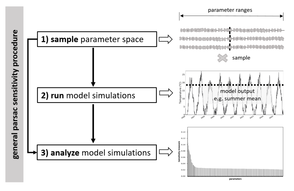
An entire parsac sensitivity process is executed in three steps:
Or as statements to the console:
where “xmlfile” is the entire path to the xml file with the SA set-up (as described above) and “pklfile” is the entire path to the pickle file being created during the sample step with the sampled parameter space, updated with model output in the run step and analyzed with the specified SA method in the analyze step.
For other options in parsac sensitivity, check the parsac help command by typing:
parsac sensitivity –h
Currently, all sensitivity analysis methods is dependent upon a specific sampling strategy. Corresponding sampling and analysis methods are:
For more details about sampling and sensitivity analysis methods, see SALib documentation (https://salib.readthedocs.io).
For more details on parsac, see https://bolding-bruggeman.com/portfolio/parsac/ and parsac Github page https://github.com/BoldingBruggeman/parsac
bat files for executing parsac sensitivity commands (optional)
Example of 3 bat files for running an entire Delta analysis with 1000 samples and a resample size of 100 when estimating confidence intervals.
PARSAC SENSITIVITY SAMPLE
C:\Python3\Scripts\parsac sensitivity sample C:\Data\lake_models\lake_example\parsac\config_parsac.xml C:\Data\lake_models\lake_example\parsac\delta_n1000.pkl latin 1000
PARSAC SENSITIVITY RUN
C:\Python3\Scripts\parsac sensitivity run C:\Data\lake_models\lake_example\parsac\delta_n1000.pkl
PARSAC SENSITIVITY ANALYZE
C:\Python3\Scripts\parsac sensitivity analyze --pickle C:\Data\lake_models\lake_example\parsac\SA_results.pkl C:\Data\lake_models\lake_example\parsac\delta_n1000.pkl delta --num_resamples 100
From the following link you can download data and files for a QWET test case. The test case is based on the Danish Lake Ravn situated in the central part of Jylland. The lake is approx. 32 meters deep with a surface area of 1.8 square kilometers.
The test case should be downloaded to follow the tutorial video "from scratch to simulation", which takes you from scratch to simulation in QWET.
If you are following one of our workshops, the follåwing supplementary material may be needed:
QWET (formerly known as WET) was originally developed by: Nielsen, A., Bolding, K., Hu, F. and Trolle, D. 2017. The original publication on the concept of WET was published in Environmental Modelling and Software. Please cite this publication when using WET:
The aquatic ecosystem core of QWET is the WET model. The WET is based on FABM-PCLake, which was developed by Hu et al. 2016, and can be cited as:
SWAT2lake - An associated tool to QWET to tailor watershed delineations with SWAT to lake and reservoir waterbodies can be found here:
This video lecture provide a brief background on the concept of WET, with focus on the individual model components, which comprise the core of WET.
The instructional videos have been created mainly to support new users of WET. The videos are voice-over screencasts that demonstrate how users can access, install and apply the software.
The "Issues" board on the WET Gitlab page effectively comprises our User Group forum. Here, you may read through the posts and answers by other users, and post your own issues or ideas for new developments.